HELP / PRIME 0.14.1
From your first spectrum to the report.
Instructions, screenshots and review criteria for Prime. Find a task, follow the application controls and preserve result provenance.
If Prime or ResinAtOnce shows “pending approval”, that copy’s request has been received, but it is not yet authorised. You do not need to create a web account or register the copy again.
Registration: what to do next, step by step → Contact public support →Start with the new contents entries: bilingual videos, lateral projection, PNG export and scientific reviews. Search also includes the earlier guide. Historical screenshots retain their version and origin; videos separately identify version, simulation or saved experimental replay. This help update neither installs another executable nor changes your project.
Watch this application’s videos →Frequently asked questions →35 chapters · search · print · expandable screenshots
Spanish and English interface and help. Step-by-step registration and approval. Screenshots of the experimental TP194 ramp. The PS conversion is exploratory and settings windows are not new measurements. Includes ultrafast D–T₂, SPEN and cancellation-recovery workflows.
No matches. Try another word or clear the search.
Registration and authorisation: before you start
DiffAtOnce Prime · This guide applies to desktop copies with access control. Registering an installation is not an online-laboratory account or a support request.
Automatic use without an initial request
The owner can enable Automatic use in Copies and installations. Compatible Prime and ResinAtOnce versions then open the workspace without an initial authorisation request, display the access mode and check the signed policy on startup and every 5 minutes. This query sends only the product and a temporary random challenge, not the copy ID, version, spectra or results. It does not accept the registration notice on your behalf or create an account.
When it is disabled, individual authorisation is checked: an active ID can continue; a pending, unregistered or blocked copy, or one without a valid authorisation, shows the access window again. A known individual block always takes priority, even in automatic mode. Offline, the automatic policy expires after 15 minutes; a valid individual authorisation retains its own expiry. A never-registered copy cannot be blocked by ID from the website until its user accepts registration. Older packages do not include this mode and retain the following workflow.
“Pending approval” confirms that the server received this copy’s registration. An administrator must review and approve it in “Copies and installations” in DiffAtOnce Studio. Continue stays disabled until the application checks an active authorisation. No approval deadline or automatic email notification is guaranteed.
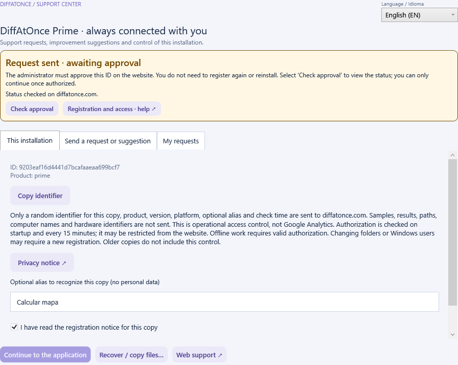
Quick steps
- In the application’s support centre, open the This installation tab. Read the notice; the alias is optional and should avoid personal data. Registration sends diffatonce.com this copy’s random identifier, product, version and platform, plus your alias if provided. The HTTPS connection uses a protected technical credential. It does not automatically send spectra, results, paths, the computer name or hardware identifiers.
- If it has not yet been sent, accept the notice and select Send authorization request. In earlier packages, the button is called Register / check authorization. Sending requests access; it does not approve the copy itself. You do not need to sign in or create a web account.
- If pending approval appears, retain this installation and its ID. You can close the window and return later: reopening restores the saved state and checks approval if the connection permits. That check does not send a new registration for an already-pending copy or approve it automatically.
- After the administrator’s review, connect to the Internet and select Check approval (or Register / check authorization in earlier packages). Continue to the application is enabled only when installation authorised appears. If it remains pending, contact support; do not repeat registrations.
- If you need help before first approval, use Web support or this guide’s public link. Integrated application support requires a previously approved copy; a later access block does not remove that support approval. In the public form, select Prime or ResinAtOnce and include the version, status and the ID provided by Copy identifier; a support enquiry does not automatically approve the installation.
Open public support → Review support privacy
If the status does not change
- Pending: await review and use Check approval. Copy identifier only copies the identifier: it does not send or approve anything. The ID is not a password; do not share identity.dpapi, secrets, credentials or spectra to resolve registration.
- Offline: a pending copy does not gain offline access. An already active copy can continue only within its still-valid signed authorisation. The default period is 24 hours from the check, configurable by the administrator; the expiry shown in the application is the reference, not a new guarantee of 24 hours after every launch.
- Blocked: retain and report the complete reason shown. Expired: connect and check again. Incorrect clock: correct Windows date, time and time zone and check online; do not turn the clock back to extend authorisation.
- Connection, certificate, signature or credential failure: retain the full message and consult support. Do not disable TLS or signature verification and do not delete the protected identity. A network error does not prove that the request arrived.
- Changing folders or Windows users: this may create another copy identity. Before moving or reinstalling, consult the update procedure or request help with the current ID. Do not clone the identity or reinstall to bypass pending or blocked status. Experimental data and projects must not be deleted to resolve access.
Videos: learn, pause and repeat
Each workflow has a separately narrated Spanish and English movie, on the website and in WPF packages that include the player. No copy registration is required to read this public help.
- Open Workflow videos and choose Prime or ResinAtOnce. Use the website language: Español plays Spanish audio; English plays English audio with its corresponding interface, poster and chapters.
- Select Play; there is no autoplay. Use chapters to return to a step and CC to select Spanish or English captions synchronized with that movie.
- Expand Steps, provenance and transcript to read or download the text. Changing captions alone does not change narration; change the page or WPF-player language for another voice.
- In the application open Vídeos de uso / Workflow videos from Help and select Español or English. If an older copy does not include these media, use the web gallery; do not download executables from unrelated links.
- Play the step, pause the video and practice in a copy of your project. Check the displayed version: buttons can be positioned differently in an earlier executable.
These are edited sequences of actual WPF captures with local synthetic narration, not continuous mouse recordings. Synthetic demonstrations and saved experimental results are labelled separately; they are neither experimental validation nor chemical identification.
2D field and lateral-projection components
The spatial Gaussian dictionary reconstructs the 2D view; its atoms are not the lateral-projection component count. Several ppm signals can contribute to the same lateral lobe.
- Select DOSY or MwOSY and Original or Model to decompose the projection. Use Residual only as a signed diagnostic, not as a positive mixture. Check protocol and source; the total blue curve is not an individual Gaussian.
- New maps automatically use lateral-modes-v1. For a saved map use Recalculate lateral-projection components and preserve the new decomposition as an explicit review. Opening a file does not replace its historical model.
- The fit detects lobes by prominence and local support and fits the unsmoothed active projection in log10(D) or log10(M). Three supported lobes can yield three components; three are not always imposed, nor is every 2D atom drawn as another lateral component.
- Review total, fitted sum, components, signed residual and positive unassigned signal on the same scale. If a broad curve covers both peaks and valleys, compare local support and Original view before accepting it.
- Advanced settings allow review of prominence, component limit and exploratory manual fitting. The standard maximum is ten, not ten mandatory components. The historical dictionary-marginal-v1 diagnostic remains separate from lobe counting.
- Select a component to inspect its ppm contributions. Recalculating the projection alone neither reinverts the signal nor changes D or reapplies standards, temperature or molecular calibration. Cancelling retains the previous decomposition.
A Gaussian lobe is descriptive, not a species or concentration. The model may declare visually added area and preserved signal: these are not new measurements. Inversion, 2D field and lateral fit have separate states; a satisfactory lateral fit does not fix a non-converged inversion.
Export DOSY, MwOSY and attenuations to PNG
Save a high-resolution figure without capturing the whole screen or recalculating the analysis. The PNG preserves the visible framing, representation and theme.
- Open the completed plot. Select DOSY or MwOSY, Original/Model/Residual, standards, component and zoom. Reset zoom first to show everything; export does not change it automatically.
- In Prime select PNG · DOSY / MwOSY… on the map. In the peak window use PNG beside attenuation, ln(I/I₀) or the calculated distribution.
- In Local signal · TRAIn / compare, after calculation, use PNG · attenuation… or PNG · distribution…. A pending plot is not exported as a result.
- The proposed size is 4800 pixels wide at 300 dpi. Choose 2400/150, 7200/600 or a custom size. Height retains the visible plot’s proportions; resize the window first for a taller figure.
- Review pixel dimensions and physical size before saving. Limits are 512–12000 pixels wide, 72–1200 dpi, 16000 high and 64 million total pixels. Increasing dpi alone does not create more pixels.
- Choose filename and folder; confirm only if you want to replace an existing PNG. Cancelling creates no figure. For an empty area or excessive-size warning, open and resize the plot, then retry with an admissible size.
More pixels improve presentation, not scientific resolution, observation count or identifiability. An image does not replace the project, contracts, parameters or report.
Distributions, moments and uncertainty: what to report
Review the distribution and its contract, not just a central D. The shared workbench supports method comparison and saved reviews without overwriting accepted results.
- Open Scientific workbench from the local signal to retain the same region, observations and factors. Compare methods with identical inputs and protocols, not a local signal against a global band summing other ppm positions.
- Check whether values are integrated bin amplitudes or densities per linear or logarithmic unit. Record units, boundaries, orientation, support and threshold. Transforming all D→M preserves integrated weights; only density transformations require a Jacobian.
- Declare number, mass or unknown signal-response weighting. Mn, Mw and dispersity depend on that declaration; M(central D) is a different quantity. Mean Rh also generally differs from Rh at mean D.
- Compare full workbench support (0%) with historical summaries that may use 1%. The figure’s visual threshold is different. Do not change historical protocols to force agreement or interpret visual Gaussian area as concentration.
- In Uncertainty document fit, gradients, standard, temperature, viscosity and calibration, with covariances and shared errors where applicable. Empty means unknown: residuals do not automatically replace independent sigma. Stability is sensitivity, not a confidence interval.
- Explicitly accept and apply a compatible review, keeping the previous one. For a whole-map family profile review equation, units and domain; applying it creates a derived review. Save the project and open the report and exported CSV/contracts to check their review and support.
Execution, convergence, noise compatibility, identifiability and experimental validation are different checks. Conditional intervals are not total uncertainty. Spectral Mn without eligible real data, joint reconstruction and rPROP remain experimental pilots; they do not establish absolute masses for stars or brushes.
Resolve a warning and report a reproducible problem
Keep the complete message and context before changing parameters. An access, drawing or export problem is not necessarily a solver failure.
- If Continue is disabled, read registration status. A pending request requires approval of that copy; a support ticket or researcher account does not authorize it. Check status again after approval.
- If Copy identifier fails with OpenClipboard, select and manually copy the identifier where possible. Do not change installation identity or delete its files to attempt registration again.
- If no attenuations are accepted, review phase, noise, signed signal, useful points, b and exclusions. Keep the previous result and attempt diagnostics; do not relax criteria just to produce a figure.
- If editing and result differ, restore saved settings or calculate a new review. Do not mix another ramp’s result with the editable selection. Retain non-convergence or unknown-noise status in the report.
- In Support and suggestions specify Prime or ResinAtOnce, version, steps, ramp/ppm region, method, parameters, factors, literal message and screenshot. Attach only a minimal authorized copy, without keys, tokens or personal or confidential experimental data.
Open Support and suggestions → · Read frequently asked questions →
Do not replace calibrations to match an expected result. TBO retains its experimental calibration; originals and historical results must not be edited to silence a warning.
A selected peak: attenuation, distribution and linear fit
First choose what you want to estimate. A monoexponential fit, a local distribution and a global-projection band are different results; they need not give the same value.
- Double-click the upper spectrum. Prime marks the measured local maximum and opens its attenuation. Check the marked ppm and extraction half-width: the same region is extracted throughout the ramp, without following each spectrum’s maximum. To compare an exact map bin, double-click inside the map or use Local signal / compare.
- Check standards, temperature and medium before calculating. This panel retains a fixed snapshot of the conditions. To change them, close it, open Prepare DOSY / MwOSY and select the signal again; Rh requires a reviewed viscosity.
- Calculate D / Mw and distribution runs the local inversion using the selected method. D only · no distribution computes a monoexponential fit and shows its D as a line: it does not create a distribution or dispersity. Review method, grid, convergence and residual before retaining it.
- Open ln(I/I₀) · linear fit and points. The all-valid-points fit and selected-points fit show slope, intercept, R² and D. NaN/Inf, invalid b and nonpositive intensities are documented as inadmissible for the logarithm; they are not clipped or removed from the original inversion.
- To explore exclusions, select Automatic · improve R², or edit Use under Points · manual selection and select Apply manual selection. All valid restores the complete diagnostic. Initial automatic-selection limits retain at least six points and 80% of the b range, removing no more than 20%; review limits and reasons, not only final R².
- Add to results and Save linear fit are separate actions; save the project afterwards. To include a workbench supplement, accept its review, open Scientific reviews, choose the target and justification, and select Apply review explicitly. A local supplement applied to a map does not replace its global inversion.
Improving R² through selection can bias D. OLS error is conditional on the selected points: it does not by itself cover selection, calibration or convection. An averaged region need not equal one bin; match observations, grid, method and factors before comparing. A nonconverged iterate remains diagnostic, not a validated solution.
Review drift without altering originals
Standard values provide a starting point; Advanced only exposes the settings. Alignment requires an independent review and explicit application.
- Check whether the header identifies standard or custom/imported values. Opening or closing Advanced changes no numbers. Saved settings remain active even when the section is collapsed; Restore standard values is an explicit action for the next calculation, not an update to earlier results.
- For a conventional DOSY ramp, select Review / align or follow Beatrix’s contextual prompt. Compare interval, anchor experiment, ppm shift, spectral shape and area-versus-b curve. Unresolved means insufficient evidence, not proven absence of drift.
- Use Advanced · alignment only when you need to review the anchor, intervals or maximum drift. After editing, select Review with these settings. Check signal loss/fill and rejection reasons; do not relax safeguards to obtain a more attractive fit.
- Select only reviewed intervals, confirm the review and record your reason. Create aligned copy retains the previous project and creates another project. Review standards and conditions and recalculate D and maps on that copy; earlier fits are not transferred and alignments are not accumulated.
iCOshift-Prime is a modified in-house variant based on iCOshift, not the complete official MATLAB version. Changing proportions of overlapping signals can resemble shifts. Alignment does not correct convection, phase, encoding or failed acquisitions, and cannot recover signal lost in noise. Do not apply this conventional route to SPEN/ultrafast without sequence-specific reconstruction.
SPEN and ultrafast: choose the correct workflow
There are two distinct routes: exploratory ultrafast D–T₂ notebook processing, and guided reconstruction with a documented kernel and calibration. Opening an example or figure runs neither route.
- Under Examples and references, review DOI, licence, manifest and hash before extracting a package into a new folder. Published SPEN-DOSY data retain their provenance. Marek 1502 is a local example: no public licence is declared and its experimental data are not distributed here.
- To reproduce exploratory processing of 1502, open Scientific workbench → Data / R&D → Ultrafast CPMG · open SER, then Process notebook / D–T₂. Review digital filtering, cropping, orientation, Gmax and chirp bandwidth; explicitly confirm the assumptions used. Retain acquisition temperature and do not copy TBO calibration from another experiment.
- Choose TRAIn2D · C# · in-house adaptation or FISTA 2D: they are different methods. Under Advanced, review the selected method’s criterion: TRAIn2D uses term_fac relative to the NNLS residual; FISTA uses its regularization and KKT criterion. Parameter changes require recalculation; a failed method is never automatically replaced.
- For the physically documented route, open SPEN / ultrafast · guided workflow. Import CPMG SER or a uniform SPEN/EPSI contract and follow Data → Echoes → Phase / axis → Profile / kernel → Inversion → Controls. Supply order and timing, spatial axis, phase, measured profile and compatible kernel before reconstructing. Do not confirm a review you cannot support.
- Inspect observed signal, prediction, signed residuals, projections and boundary accumulation. In the guided workflow, compare against a conventional DOSY control from the same preparation and conditions, with tolerance declared before comparison. Save the workflow and export result and provenance; adding it to the project/report requires explicit review.
CPMG retains echo time: its map is D–effective-T₂, not ppm–D. SPEN/EPSI requires its own contract; the published external SCORE reproduction is not presented as native Prime output. Example 1502 does not itself supply a measured coil profile or validate b, quantitative D, MwOSY, a new sequence or single-scan acquisition. Meeting a numerical stopping criterion does not establish identifiability or experimental validation.
01 · Choose a product and start
Prime is the general-purpose diffusion workspace. ResinAtOnce retains the resin-specific workflow.
- Open your existing Windows Prime package; check the executable version. This website does not enable a new public download.
- Open Bruker data or a .prime.json project. Use Synthetic demo only to learn the interface.
- Follow acquisition → preparation → calculation → review → save → report.
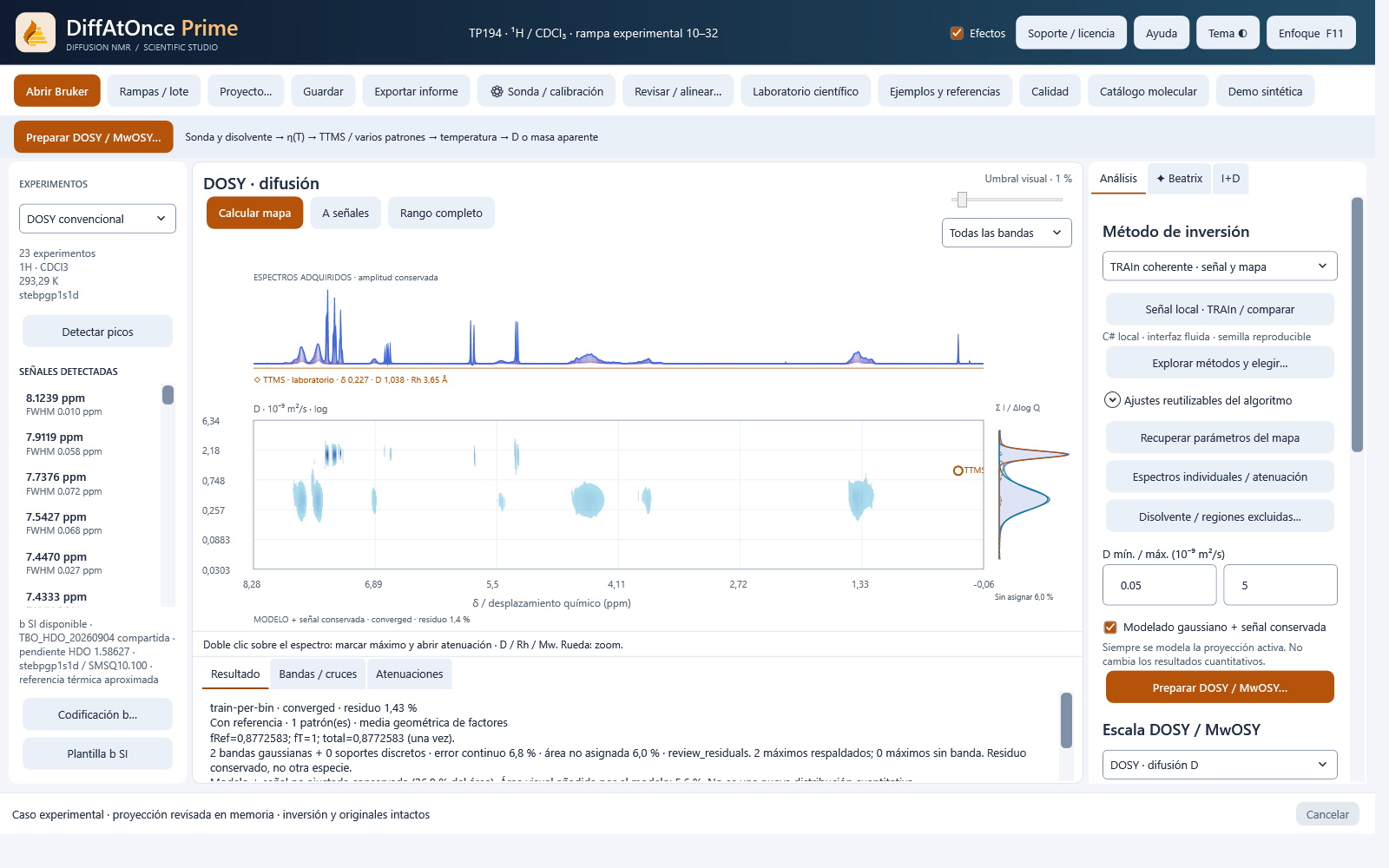
23 experimental TP194 spectra in CDCl₃; ramp 10–32. Saved TRAIn map, TTMS standard and active projection. Residual and status describe this calculation, not universal validation.
A general-purpose interface does not make molecular calibrations universal. Review each model’s medium and domain.
02 · Import a Bruker ramp
The conventional DOSY import route reads processed 1r spectra, retaining amplitudes and metadata.
- Select Open Bruker and the acquisition with numbered experiment folders. Set ramp, pdata number and points per bin.
- Review title, nucleus, solvent, sequence, TE, RG, NS, probe and gradients. Do not combine incompatible acquisitions.
- Use binning 1 to retain full resolution; binning speeds up calculations but changes the averaged region.
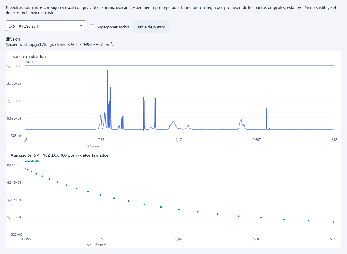
Measured spectra and local region. Common scaling and signal sign are retained; experiments are not individually normalised to match.
The ultrafast D–T₂ module has a separate raw-data and echo-contract route. This is not a universal FID/ser processor or automatic SPEN reconstruction. Originals are unchanged.
03 · Navigate, zoom and change theme
Spectrum, map and projection share context; the side panel holds the controls.
- Use Theme ◐ for light/dark and Focus F11 to give the map more space. Effects can be disabled.
- Fit signals frames visible bands; Full range restores the entire axis. Use the wheel to zoom.
- The visual threshold is at the upper right. Change Original/Model through representation settings.
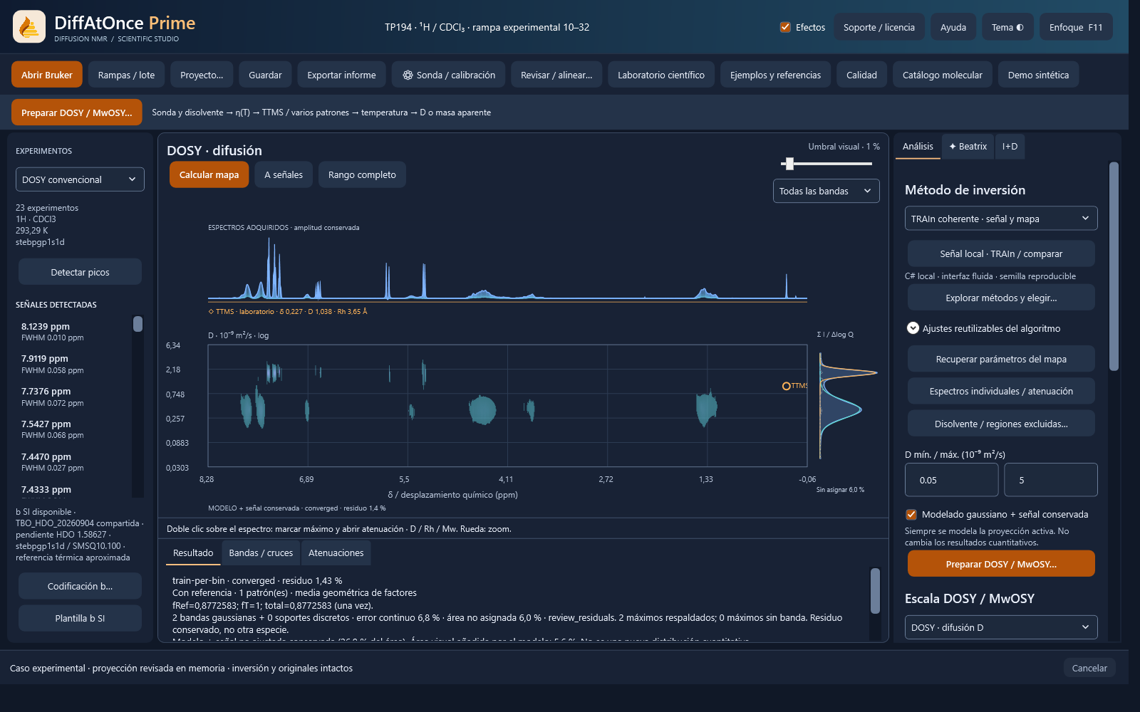
Changing theme does not change intensities, calibration, representation or results.
Zoom, theme and threshold are display controls: they must not change the data, selected representation or quantitative moments.
04 · Probe and b encoding
Probe detection and gradient calibration are separate decisions.
- Open Probe / calibration. Automatic reads PROBHD; a documented manual label is also available.
- Retain reviewed b or import a b manifest in s/m². You may also review Gmax or calibrate with a known solute in the same medium and temperature.
- Preview factors and b by experiment, document the source and apply to a derived copy. Recalculate afterwards.
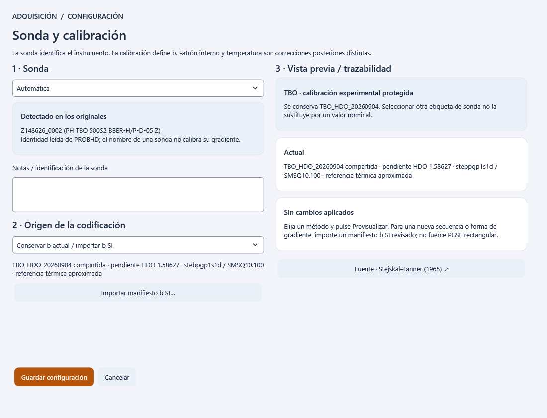
Calibration window for the real case; no changes applied. A probe label does not determine Gmax.
The rectangular PGSE formula is not valid for every sequence. The shared experimental TBO calibration is protected; a detected probe does not authorise nominal Gmax.
05 · Solvent, temperature and viscosity
Open Prepare DOSY / MwOSY → Medium / temperature.
- Check detected SOLVENT and TE. Select an available correlation or enter manual viscosity with source and Pa·s units.
- Use fixed η at a reference temperature (293 K proposed) or temperature-dependent η. Confirm applicability to your composition.
- Thermal normalisation of D is a separate option: choose output temperature and law. Check factors before applying.
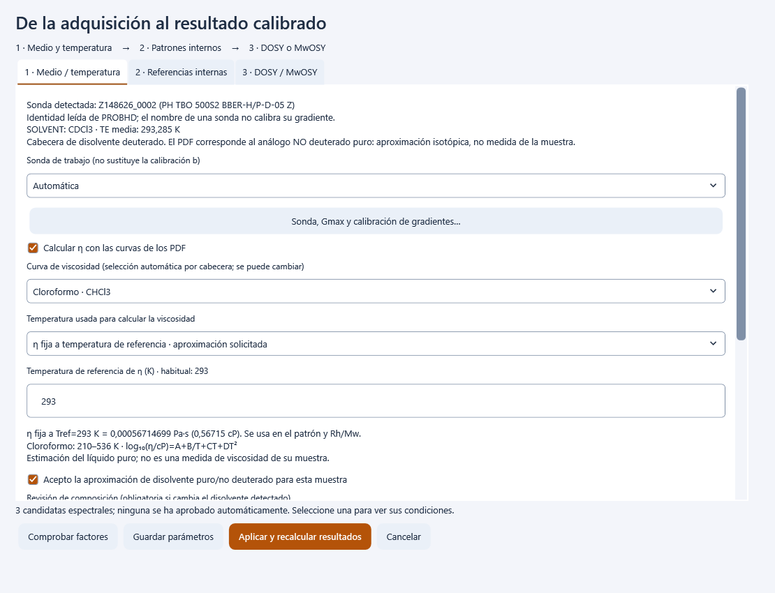
Settings for the real acquisition. Pure-solvent viscosity is a reviewable approximation, not a measurement of the mixture.
The ten solvent curves come from the documented package sources. A pure/non-deuterated analogue does not measure the viscosity of a concentrated mixture. Rh requires reviewed η.
06 · TTMS and multiple internal standards
Detecting a signal does not mean approving a standard.
- Open Internal standards and select Detect / recheck. Review position, attenuation, local D and documented Rh.
- Confirm which substance you added and its region. The laboratory TTMS protocol uses Rh = 3.65 Å, conditional on identity and medium.
- If expected D is missing, review η(Tref) beside the standard. For multiple standards, use Manage multiple and check compatibility before enabling them.
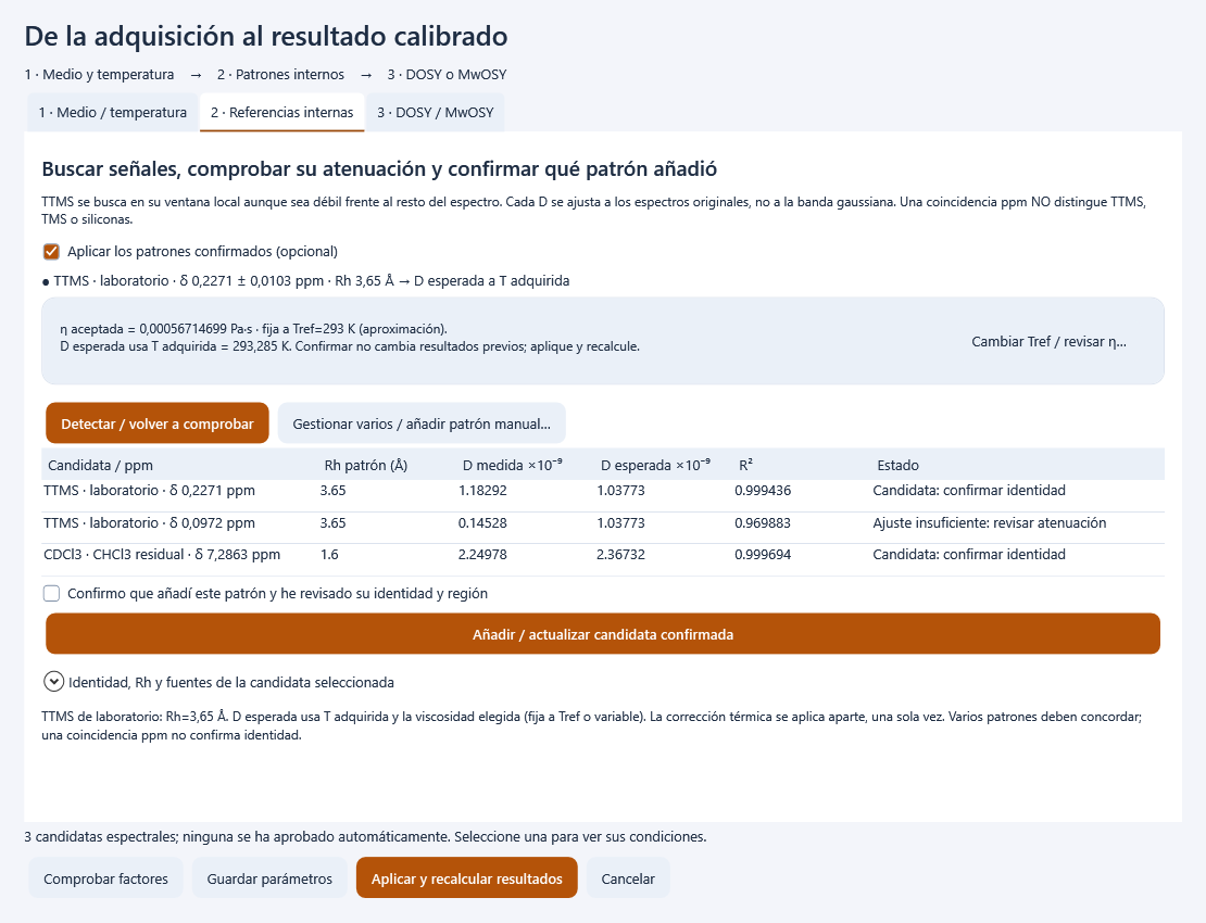
Detection on the real ramp and saved settings. A ppm candidate does not confirm which substance was added.
Compatible factors are combined; overlapping or discordant standards require review. Do not force each standard to its expected value using individual factors.
07 · Calculate without an internal standard
An internal standard is optional, not a prerequisite for D.
- Disable Apply confirmed standards or choose the no-internal-standard mode.
- Review b, temperature and remaining assumptions; recalculate.
- Check WITHOUT INTERNAL STANDARD in the result and report. Standard definitions can remain saved.
Unchecking a box does not retroactively remove calibration from a saved result. New settings take effect when recalculating.
08 · Apply corrections without duplication
Prime retains measured D, fReference, fTemperature and their product.
- Use Check factors to preview. Save parameters does not replace the previous result.
- Apply and recalculate archives the previous state and recalculates maps and regions with the same settings.
- Review final D = measured D × fReference × fTemperature and the associated conditions.
A temperature correction is not a convection correction. Do not use the same solute to calibrate b and correct D again without checking double counting.
09 · Calculate DOSY and select a method
Calculate map uses edited method and conditions; the previous map retains its own.
- Choose coherent TRAIn, MF-NNLS256, TRAIn-MF, RAI-S, DOME-S, SILT or the local Diffusion-Inversion route for your problem.
- Review ppm interval, D range, bins, iterations and regularisation. TRAIn uses termFac; it is not the same parameter as λ.
- Calculate and inspect convergence, residual and attenuations. Use Cancel to interrupt; the last complete result is retained.
23 experimental TP194 spectra in CDCl₃; ramp 10–32. Saved TRAIn map, TTMS standard and active projection. Residual and status describe this calculation, not universal validation.
Different methods optimise different objectives and may disagree. Do not change parameters just to get a convergence flag or force equal bands.
10 · Omitted or rejected attenuations
The detector evaluates noise, useful signal and attenuation coverage.
- Open Attenuations. Check whether a column is continuous, discrete, a standard, excluded or omitted, and read its reason.
- If no attenuations are accepted, select a diagnostic row to inspect its exact points and noise estimate.
- Review phase, baseline, region and b; save the diagnostic. Adjust policy only with experimental justification.
An empty map is not saved as a result. Attenuation that disappears too early does not thereby contain enough distribution information.
11 · Double-click: calculate a specific peak
The marker identifies the local maximum in the lowest-b spectrum; extraction stays fixed throughout the ramp.
- Zoom into the region and double-click the peak. Check the marker and extraction half-width.
- Calculate D / Mw and distribution runs inversion. D only gives a monoexponential fit, not a distribution.
- Review the values and use Add to results; then save the project.
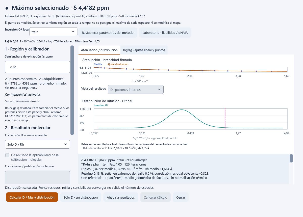
Experimental region centred at 4.4182 ± 0.04 ppm. TRAIn is calculated on original signed data; standards are markers with no area.
A different maximum is not followed in each experiment. A monoexponential D marker is not turned into an invented distribution curve.
12 · ln(I/I₀) and linear regression
The linear tab is available before inversion.
- Open ln(I/I₀) · linear fit and points. Read slope, intercept, R², measured/final D and OLS error.
- Review I₀ and b₀: they come from the positive point at the lowest available b. The horizontal axis is (b−b₀)/10⁹ and the intercept is free.
- NaN/Inf, invalid b or I≤0 are excluded only from the logarithm, with a reason in the table.
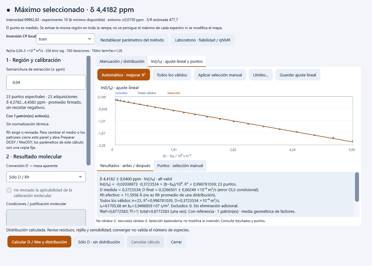
OLS fit to every valid point in the experimental region. I₀ is the positive intensity at the lowest available b.
Log-space OLS and intensity fitting minimise different errors. OLS error excludes calibration, selection and convection uncertainty.
13 · Automatic and manual point selection
Review compares all valid points with the selected subset and keeps exclusions visible.
- Automatic · improve R² searches within limits: by default ≥6 points, ≥80% b coverage and ≤20% valid-point exclusions.
- For manual decisions, select rows and press Apply manual selection. All valid restores the baseline fit.
- Save the linear fit to include it in the project and report, with mask, reasons and comparison.
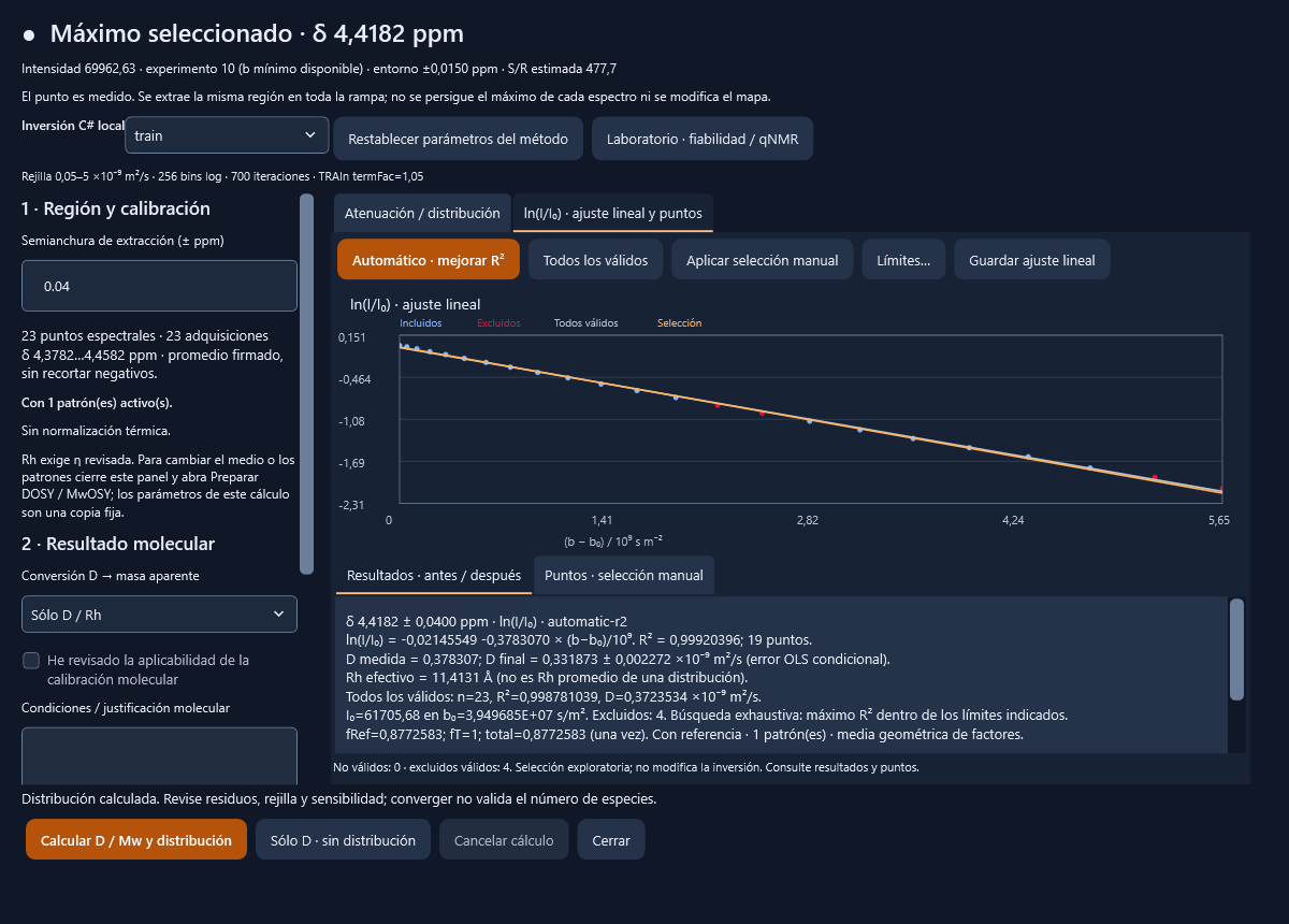
Exploratory R²-based selection. Excluded points remain visible; the mask does not affect inversion or the map. Higher R² does not prove a more accurate D.
Improving R² may bias D. Selection is exploratory, not proof of absent convection or an automatic mask for TRAIn, Tikhonov or MaxEnt.
14 · Distributions, regularisation and components
A 1D distribution describes a specific region; it is not the projection of the entire map.
- Select local method, grid and parameters. Reset parameters proposes values; it does not validate their optimality for your sample.
- Compare signal/prediction, residuals, boundaries and sensitivity to λ or termFac. A non-converged iterate is diagnostic.
- In Separate components, review valleys, descriptive Gaussians, residual and component moments. Original bins are retained.
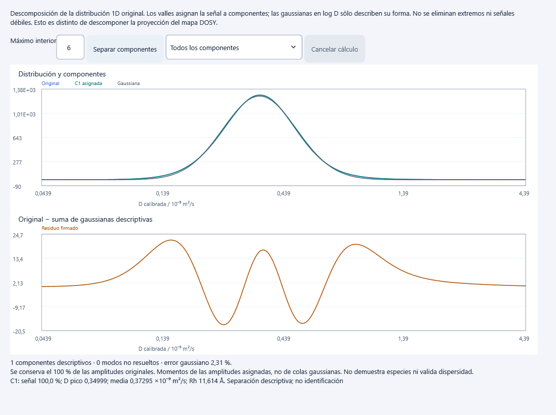
Descriptive separation of the calculated distribution. Moments use assigned bins, not Gaussian tails or identified chemical species.
The number of modes depends on resolution and regularisation. It is not the number of compounds or their concentrations.
15 · Compare local TRAIn and DOSY
Use Local signal · TRAIn / compare to inspect the original bin and its settings.
- Select the same interval, ppm binning, acquisitions, b, method, grid and parameters.
- First compare measured D and original distribution; then fReference and fTemperature.
- Distinguish local components, MF rank and global-projection bands. They are different objects.
A difference between a global band and a local region is not itself an error. Numerical agreement requires identical inputs and objectives.
16 · MwOSY: choose the molecular calibration
Changing the axis does not turn apparent mass into validated absolute mass.
- In Prepare DOSY / MwOSY → 3 choose D, high-dilution PS, high-dilution PPG, shared concentration or a custom curve.
- PS and PPG are two high-dilution curves. There is one concentration model, developed with PS; it does not depend on choosing PS/PPG.
- Review viscosity, temperature, conditions and domain. The shared implementation requires ¹H/CDCl₃ and output near 293 K; other media require a custom calibration.
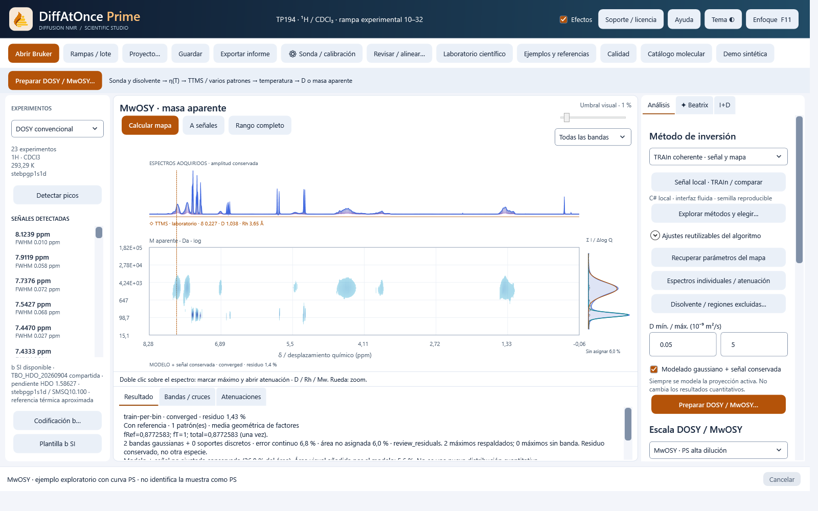
MwOSY view derived from the experimental map with the high-dilution PS curve. An apparent-mass conversion example: it does not identify TP194 as PS or validate its absolute mass. No weighing data were invented.
A small standard calibrates D, not the D–M relation of every polymer, star or brush. The PS screenshot is an exploratory conversion, not the sample’s identity.
17 · Weighings and concentration
Only the concentration model needs C = solute mass / solvent mass, in mg/mg.
- Prime looks for masses with units in the title of the first experiment in the ramp. They may occur anywhere in the text.
- The first is solute; the second is solute + solvent. Subtract them to obtain solvent. mg/g and decimal comma/point are supported.
- If information is missing or ambiguous, fields remain empty. Enter both weighings or explicitly review a historical C; zero is not invented.
Arithmetic example, not screenshot data: 7.52 mg and 827.09 mg → 819.57 mg solvent → C ≈ 0.00917554 mg/mg. This is neither percent nor mg/mL.
18 · Gaussian field and active projection
Modelling is descriptive and retains positive unfitted signal.
- Gaussian modelling + retained signal is enabled by default. Change it in advanced settings.
- The projection is recalculated from the active representation. Review error, visually added area and model residual.
- Select a projection band or map cross-peak. Inspect peak, mean and Rh or mass moments for the complete band.
Gaussians and bands do not prove chemical species. Visual threshold and band selection must not erase original signals or change saved results.
19 · Review and apply alignment
Beatrix flags possible shifts; the application never aligns without review.
- Open Review / align and compare intervals, experiments, shifts and before/after attenuation.
- Adjust anchor and limits if needed. Unresolved means the method lacks sufficient evidence to shift that case.
- Confirm your reason and create an aligned copy. The previous state is archived; review standards and recalculate results.
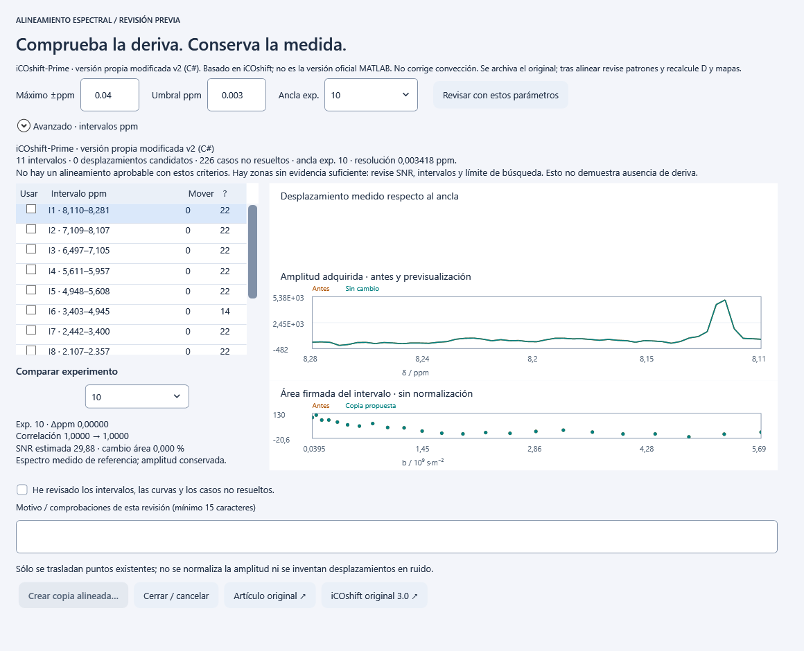
iCOshift-Prime review of the experimental spectra; no alignment applied. Unresolved cases do not mean there is no drift.
iCOshift-Prime is a modified in-house C# version, not official iCOshift 3.0. Alignment neither corrects convection nor validates overlapping-component areas.
20 · Convection diagnosis and review
Diagnosis distinguishes detected, not detectable and inconclusive.
- Select the signal and open R&D → Analyse ramps from this preparation. Compatible ramps and known calibration are required.
- Read Guide and final correction: noise, sequence moments, stability and sensitivity must meet the requirements.
- Where eligible, calculate physical inversion or document another control acquisition. Explicitly activate the final revision for that signal.
The entire map is not automatically rescaled. The report distinguishes physical correction, another control measurement and no correction. High R² does not rule out convection.
21 · Beatrix and assignment suggestions
Cards start from the same peak, band and result you are viewing.
- Hover over a signal to see hypotheses. Click to pin context and open cards and sources.
- Review nucleus, solvent, accompanying windows, multiplicity and other band cross-peaks. Open the source before assigning.
- History is labelled historical. Pause prompts or configure local AI/API providers; keys are not part of the project.
- Local inference requires matching model, corpus and manifest. A checksum mismatch blocks that inference; rules and documentation remain available. Use a matching package; do not disable the check or attribute rule-based guidance to an LLM.
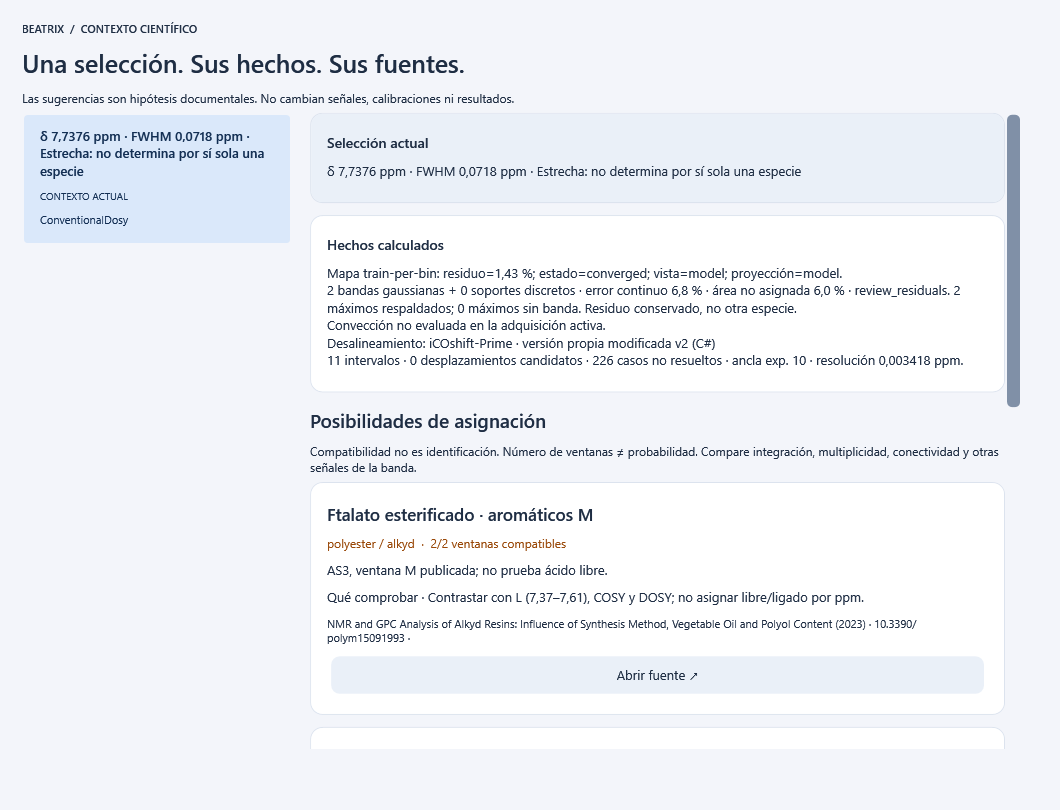
Experimental aromatic region. Documentary suggestions, such as a phthalic fragment, require checking other signals; they are not automatic identifications.
AI integrated into the workflow, with visible context
Beatrix connects the selected signal or band, calculation-engine facts and available sources to guide the next review. It can help explain what is missing when preparing a ramp, how to compare a fit, or which check to document before a report. Computed facts, rule-based recommendations and generated text are distinguished: it is not an alternative calculation engine.
Choose capacity for your computer and configuration
- Local rules: contextual guidance without an LLM or data transfer. This is useful when no model is configured; it is not presented as AI inference.
- Local CPU: configure GGUF CPU, the model path and its SHA-256. Small, medium and large profiles support different response budgets and user-configured models. The model must fit available RAM; CPU and model size affect speed. Choosing a larger profile does not automatically download, train or install a model.
- Compatible server / API: configure the provider, URL, accessible model and, where required, the key environment variable. A GPU is used only if the configured server provides it; owning a GPU does not activate native GGUF CPU acceleration. A remote endpoint requires HTTPS and explicit permission to send context. Review the context and provider terms before asking.
Check the response for the provider and model actually used. More capacity may broaden or speed up an explanation, depending on model and hardware, but does not by itself make calibration, assignments or experimental results more reliable. Better hardware does not automatically select a more powerful model.
Five examples of questions during analysis
These are illustrative workflows, not calculated answers for a sample or new experimental evidence. First select the context your question refers to.
- Import and calibration — “What should I check before calculating this ramp?”. Check the spectrum, title, sequence, gradients/b, probe, solvent and temperature. Beatrix guides encoding and standard checks; you review expected D, viscosity and the factors to be applied. Do not confirm TTMS solely because it is near 0 ppm.
- Hover and assignment — hover over a peak and click to pin it: “Which hypotheses are compatible, and which companion signals are missing?”. Review cards, sources and conditions. In 1D / 2D evidence you can enter COSY/HSQC/HMBC cross-peaks actually observed in the same preparation; Beatrix reuses reviewed evidence without turning a match into a confirmed identity.
- Possible misalignment — “Should I review this signal’s shift along the ramp?”. If prompted, open Review / align and compare intervals, shifts and before/after attenuation. Only your review and confirmation create the aligned copy. Beatrix does not align independently, and alignment does not correct convection.
- Fit and residuals — “What should I check if the residual is structured or the method does not converge?”. Open the attenuation and compare prediction, signed residual, b coverage, exclusions and settings for the same bin/region. Beatrix explains the available diagnosis and can point to Scientific workbench for method and stability comparison; it does not turn high R² into scientific approval.
- Next step and report — “What still needs documenting before sharing this result?”. Review measured versus corrected D, standards, temperature, viscosity, mass model and limitations. Save the justified review and check the project and exported report. Accepted supplements retain their provenance; advice does not replace or edit a saved result.
The catalogue contains polymer/resin fragments and impurities, not all chemistry. A match is neither identification nor probability. GPU/API connectivity depends on the provider; no newly validated fine-tuning is claimed.
22 · Local library, HTTP and external algorithms
Local Diffusion-Inversion and an HTTP connection are different routes.
- The local selector runs the bundled C# library without an HTTP server or MATLAB. Review parameters for each method.
- For HTTP, configure the endpoint and JSON/SI contract. Review data leaving the computer and authorise the request.
- An external executable requires path, arguments, hash and timeout. Inspect the response before using it.
Not every endpoint or executable is compatible. External results are not automatically applied to the map or considered validated because they came from an API.
23 · SPEN, ultrafast and provenance-tracked examples
Each modality has its own data, sequence, contract and limits; no universal reconstruction is claimed.
- Open Examples and references: SPEN-DOSY and UF-DEXSY include publications, repositories, licences and SHA-256. Local ultrafast example 1502 includes user-supplied raw data and code without claiming a publication of its own.
- SPEN-DOSY is inspected as a published package; its spatial reconstruction is not a native Prime method. UF-DEXSY studies diffusion/exchange and must not be treated as ppm–D DOSY.
- For ultrafast D–T₂ use the specific workflow in the following chapter. The user’s new ultrafast DOSY sequence remains untested: do not silently substitute conventional b for its contract.
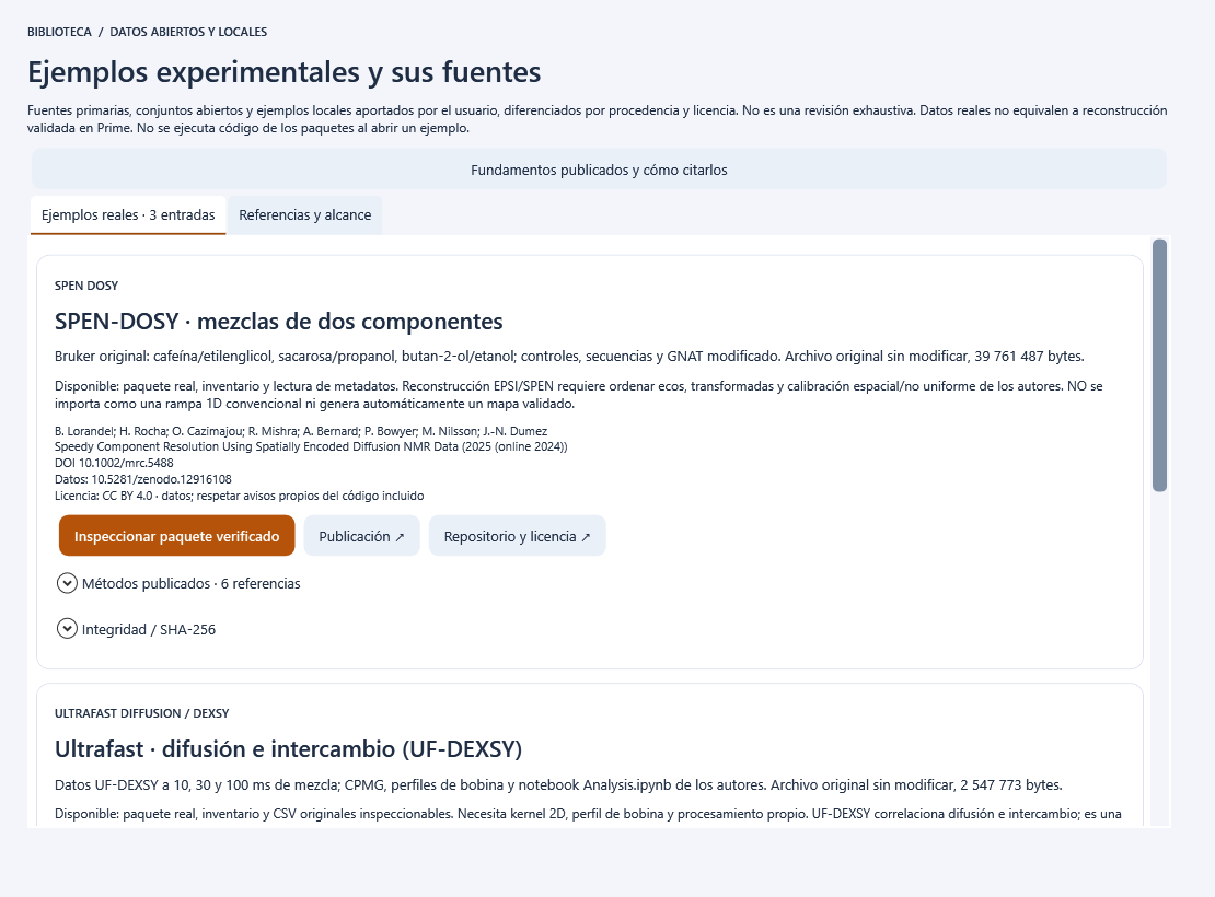
Library of published SPEN-DOSY and UF-DEXSY packages with DOI, licence and hashes, plus local ultrafast D–T₂ example 1502 with code and acquisition contract. Opening the library does not run reconstruction.
A figure reproduced with author tools is external, not a screenshot or native Prime solution. Inspection, numerical execution and experimental validation are different kinds of evidence.
24 · Batches, projects and reports
The saved result, not a pending edit, is the basis of traceability.
- In Ramps / batch choose ramps and review each set of conditions.
- Save the .prime.json project. Reusable settings retain algorithm parameters, not sample identity or transferable calibration.
- Export report creates a new revision with editable DOCX, HTML, CSV and JSON; PNG from the view, a manifest and completion marker. Check completion before using a batch.
If editing and result differ, recover map parameters or recalculate. Do not mix another ramp’s result with the current selection. Review the report before sharing it.
25 · Ultrafast D–T₂: TRAIn2D and FISTA
The native C# module separates diffusion and effective T₂, not chemical shift and diffusion.
- Open example 1502 or compatible raw data through the ultrafast module. Review nucleus, temperature, echo count, complex points, acquisition order, spatial window and reference profile.
- Check spatial-transform and b assumptions before inversion. Example 1502 lacks a measured coil profile and uses an exploratory window; its scale is not presented as final quantitative calibration.
- Choose TRAIn2D or FISTA, review D/T₂ grids, stopping, residual and parameter sensitivity. Save contract, parameters, data provenance and output separately.
T₂ is effective and may include diffusion during readout and other effects. The example has NS = 16: it is not described as single-scan acquisition. Do not use its results as identification, calibrated MwOSY or validation of a new sequence.
26 · Audit and safe recovery
Prime 0.12.5 and ResinAtOnce 0.48.1 share tested scientific-core and calculation-state fixes.
- After a failed or cancelled attempt, check status and selection before adding results. Do not attribute an earlier graph to the new attempt.
- Local separation requires a positive increasing D grid and finite nonnegative weights. Invalid data produce a diagnostic, not a negative-area component.
- Review JSON files use atomic replacement, with a .bak copy when replacing an existing file. Keep the manifest and check the final file; cancellation is not a new result.
The empirical concentration model retains its κ(M) segment change at 117,000 Da. It does not interpolate across the gap not represented by that formula. Regression tests check specific software cases; they do not validate every sample, every method or absolute masses.
Before communicating a result
- Correct sample, ramp, region and method.
- Measured D and factors separated; standard use or absence visible.
- Mass model, viscosity and concentration documented.
- Convergence, residuals and convection reviewed; hypotheses not presented as identities.
- Project saved and DOCX/HTML checked.
WATCH, PAUSE, REPEAT
Learn with workflow videos.
Six workflows with separately narrated Spanish and English movies, in the application and on the web. Page language selects the voice, interface and timeline; CC offers ES/EN captions. Chapters and downloadable steps. No autoplay or external providers.
DIFFATONCE / MOLECULAR DIFFUSION